Levana Well-funded Perpetuals Whitepaper

Abstract
1. Motivation
- 1.1. Problems with constant-product virtual AMM model
- 1.2. Benefits of Well-fundedness
2. High level protocol overview (TODO: better drawings)
3. Trading Mechanics
4. Incentivization structure
5. Liquidity Providers
6. Delta Neutrality Fee
7. Liquidations
8. State Staleness and Cranking
9. Crypto denominated markets and off-chain notional
10. Risks, rewards, guarantees and fee size

Abstract

Levana Well-funded Perps is a leveraged, well-funded and collateral-settled perpetual swaps protocol. It introduces a novel way to delineate risk between market participants. The incentive structure offers risk premium to the liquidity providers taking on the spot market illiquidity risk. Some of its key features are:

Strong guarantees for settlement: Traders get strong guarantees for settlement in any future market conditions with a very low liquidation margin ratio. Liquidation price is solely based on spot price feed.
Risk premium for liquidity providers: Liquidity Providers receive a risk premium for taking on spot market meltdown risk. This yield is found in a free market of supply and demand for liquidity to be used as collateral.
No risk fund: Protocol doesn’t require a risk fund and the DAO Treasury has no insolvency risk.

The absence of native price discovery in spot-price settled perps is addressed by introducing a Capped Delta Neutrality Fee mechanism.

1. Motivation

1.1. Problems with constant-product virtual AMM model

A popular model for perpetual swaps is the constant-product virtual AMM (vAMM). This model introduces a virtual market against which users can trade. To ground it in reality and keep the virtual market’s price (known as the mark price) in line with the spot price, the protocol relies on a special payment referred to as a funding payment. This payment incentivizes traders to balance out long/short interest and keep the price stable.

This design was innovative and allowed for a perpetual swaps DEX to exist without an order book. However, it has critical flaws that prevent it from functioning long term in anything but a calm, low volatility market.

At the core of these flaws lies the fact that the vAMM model has unfunded liabilities. To pay out the profits to a particular trader, the vAMM model depends on two things:

Liquidating other trader’s positions before they go into bad debt.
Ensuring that certain positions remain open to keep the mark price close to the spot price.

This problem is usually solved with high liquidation margins, a reliance on off-chain liquidation bots, capital controls (such as disallowing withdrawals, closing and delisting markets, etc.), and heavy-handed dynamic fee incentives in the form of uncapped and sensitive funding rates. While these solutions work to mitigate some of the problems, they do not address the core issue, which is accentuated by the fact the protocol must still maintain an imbalance of open interest.

The magnitude of the imbalance is equal to the notional size of a position that would move the vAMM price from the price it was initiated at to the current spot price. This imbalance generally grows with time, especially in a market meltdown or melt-up. The initial vAMM price can be moved, but it is very costly to the protocol and doesn’t work in a meltdown scenario.

As the imbalance grows, so does the protocol’s unfunded liabilities. The protocol simply owes more to the popular side than it has locked in from the unpopular side. At this point, a race scenario is created whereby traders on the popular side are incentivized to close their positions quickly to ensure that they realize all of their profits. As the protocol is drained, it accrues bad debt and heads towards insolvency.

The vAMM model is brittle and has an open interest imbalance risk reminiscent of an algorithmic stablecoin depeg risk. Piling up additional incentives or market participants on a fundamentally flawed model does not inspire confidence. Because of that, Levana went back to the drawing board to design a leveraged perpetual swaps financial model that is well-funded as a core principle.

1.2. Benefits of Well-fundedness

A trader’s unrealized profit is a liability to the protocol. That liability is well-funded when the maximum profit is locked for specifically that position. By making all positions well-funded, the protocol gains the following benefits:

Traders are guaranteed a fair settlement payout in any market conditions.
Bad debt is impossible for a position by construction.
Without bad debt, there is no risk of insolvency to the protocol as a whole.
There is no rush to perform liquidations just-in-time before the position goes into bad debt.

The collateral that is locked as maximum profit comes from liquidity providers. Liquidity providers take on the risk of spot market meltdown. For taking on this risk, they receive a borrow fee with a risk premium.

The benefits of this mechanism are:

This mechanism creates a decentralized supply-and-demand free market for liquidity with yield denominated in the collateral asset.
The protocol does not have to rely on inflationary token emissions to attract liquidity.
Different listed trading pairs are completely separated from each other with their own liquidity markets. This ensures that there is no contagion risk between different markets.
Having completely independent markets makes deploying cross chain simple, as there is no risk fund or basket of notional assets that needs bridging.
Well-fundedness guarantees to traders’ positions enable fearless composability of other financial protocols on top of tokenized positions.

2. High level protocol overview (TODO: better drawings)

Levana Well-funded Perps is a platform for leveraged perpetual trades. It has multiple completely separate listed markets, each of which is a trading pair of a notional index and a collateral crypto asset.

A trader that wishes to enter a position provides collateral and gains leveraged exposure to the notional index price. All traders are guaranteed to be able to close their positions, settling with the oracle spot price. The oracle spot price is the current exchange ratio between the notional index and collateral asset.

Markets are generally separated into two categories: stablecoin denominated and crypto denominated:

A crypto denominated market has US dollars as the notional asset and a volatile native or bridged asset as the collateral asset in which every trade is opened and settled. Crypto denominated markets are well-suited for native to chain crypto assets and bridged assets with deep liquidity. Trading pairs with native crypto collateral assets do not have stablecoin depeg, centralization or bridge hack risks, and create sought-after crypto-asset lending with fair risk-premiums.
A stablecoin denominated market has a stablecoin set as its collateral asset and any notional index. Stablecoin denominated pairs are well-suited for small-cap crypto assets that are not bridged to the platform’s chain and off-chain assets. These trading pairs make it possible to list any exotic, non-crypto, or synthetic asset and create delta-neutral stablecoin lending with fair risk-premiums.

2.1. Trader’s position

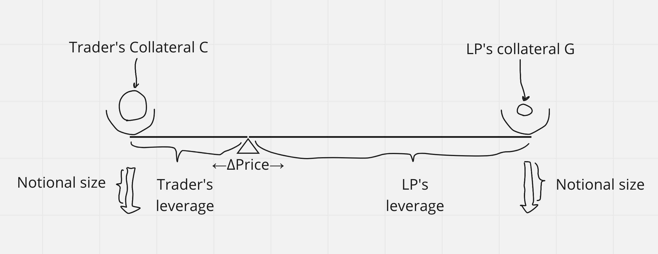
Figure 1. Leveraged position on Levana Well-funded Perps. TODO: notional size arrows should be reverse of each other. Add fee arrow directions.

Traders open positions by providing collateral and choosing position parameters. In a crypto denominated pair, the traded crypto asset itself acts as collateral, while in the stablecoin denominated pair, that stablecoin acts as collateral.

Position parameters are:

Leverage of the trade. Leverage and provided collateral (with entry price) define the notional size.
Max gains that this position can realize. This defines the amount of collateral that will be locked on the counter-position of the trader’s position. Long positions in a crypto denominated trading pair have an option of infinite max gains.

💎 Internally, Levana Perps uses max gains to define how much counter collateral to lock against a position. However, the web frontend does not expose this concept. Instead, it exposes the more familiar concept of a take profit price. The frontend is responsible for calculating the amount of max gains necessary to ensure the specified take profit price.

The collateral that the trader provides defines the max loss to the trader. The collateral that the protocol locks in the counter-position defines the max profit to the trader.

In a crypto denominated pair, long positions may have unlimited max profit if the locked collateral for the counter-position is equal in size to the whole notional size of the position.

Max loss of a position is realized when the oracle price feed crosses a liquidation price threshold. Similarly, max profit is realized when the oracle price feed crosses a take profit price, if present.

Traders may close their position at any point in time, settling the payouts to themselves and Liquidity Providers at the current spot price.

💎 All positions in Levana Perps are well-funded. Well-fundedness is a guarantee to settle at any time, at any spot price, and in any market conditions.

A trader may be unable to open a new position that would use more collateral on the counter-side than the liquidity remaining in the pool of available capital. This is expected to happen only in extreme market conditions.

2.2. Liquidity Providers’ pool of capital and yield

Liquidity Providers deposit their funds into a single pool of capital denominated in the collateral asset of the trading pair. This pool is specifically for that trading pair, and funds from it are used to enter into a net total counter-position to all traders’ positions for that trading pair.

To make the liquidity pool roughly delta-neutral with respect to the notional index, the protocol charges a per-block funding rate fee from owners of popular-side positions and pays this to owners of unpopular-side positions. The payment is scaled with signed notional size of the position.

To compensate Liquidity Providers for the cost of their capital and a premium on the risk that they take on, the protocol charges a per-block borrow fee from all traders and pays it to Liquidity Providers as yield on provided principal.

🔥 Liquidity Providers take on the risk of the meltdown (or melt-up) of the assets, but not a bear (or bull) market. The difference between meltdown and a bear market of the same magnitude is the existence of cash-and-carry traders comfortable enough to perform arbitrage to earn funding rate payments, bringing the LP pool into rough delta-neutrality.

2.3. Protocol Market Participants and Incentives schema

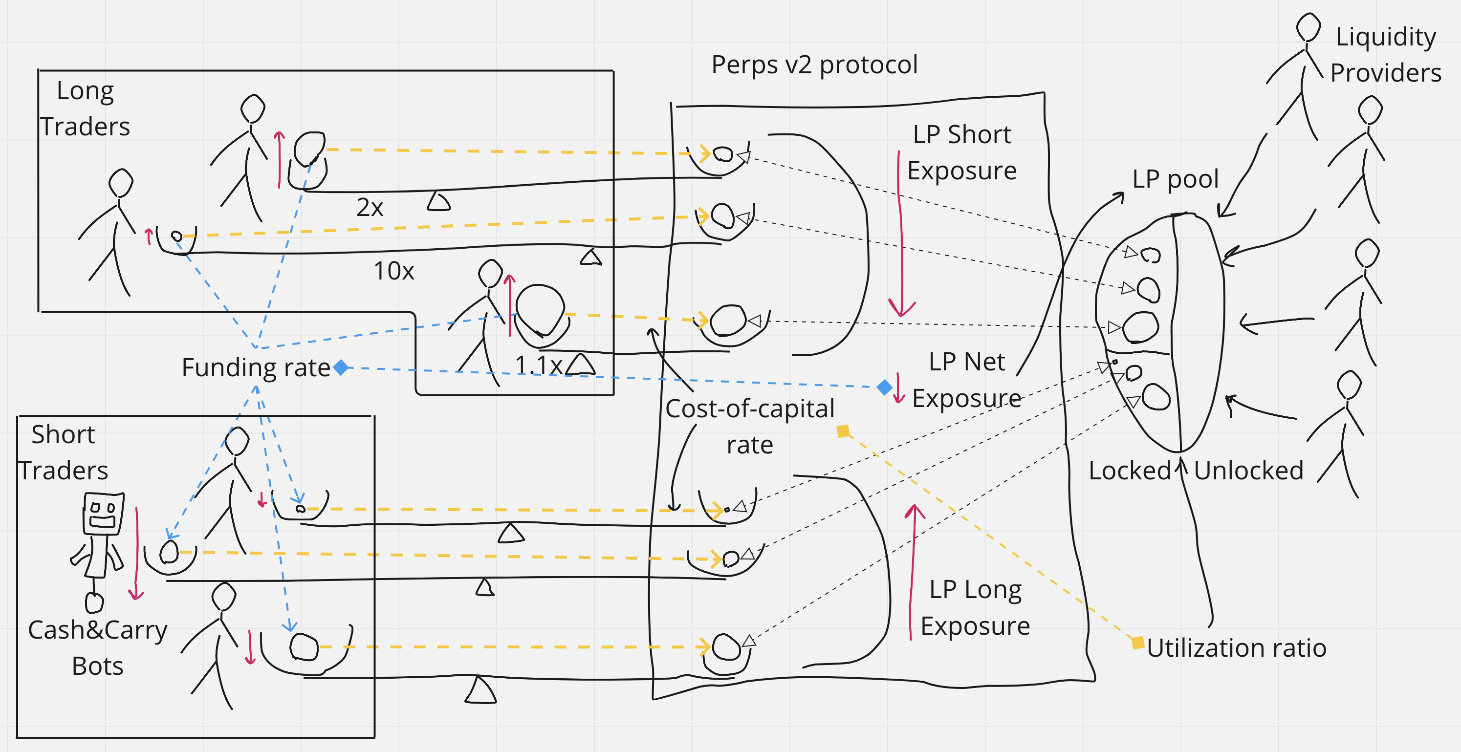
Figure 2. Market participants and protocol balancing on Levana Well-funded Perps. TODO: Borrow fee yellow lines should go into a separate yield fund, not collateral on the counter-side. Add delta neutrality fund to the schema?

Funding payments are paid from positions with popular directional exposure to the unpopular ones. The funding rate is scaled with net notional open interest. The funding payment for a particular position is scaled with notional size of that position.

Cash-and-carry bots come to earn funding payments. To do that, they open unpopular positions on Levana Well-funded Perps, and also open counter-positions on the spot market to become delta-neutral.

For crypto denominated pairs with collateral assets that have high staking rewards, there is also a unique delta-neutral strategy available on Levana Perps that allows traders to earn staking rewards without exposure to the underlying asset. This possibility exists because it is possible to open a short position that pays a borrow fee on a fraction of the notional size of the position.

Liquidity Providers pool their capital into a single liquidity fund per market. This pool of funds is used to lock collateral on the counter-sides of all traders’ positions. The fund has a utilization ratio of locked funds to all funds in the pool. Borrow fee payments are payed for locked collateral on the counter-side and appear as yield for Liquidity Providers. A part of the yield stream goes to the protocol treasury.

2.4. Protocol dynamics listing a high staking rewards token

The unique feature of Levana Perps is that traders pay a borrow fee on counter-side collateral, which can be multiple times lower than the notional size of the position. This gives traders the ability to hedge high staking reward tokens cheaply, making it viable to earn delta-neutral yield from staking.

Because the delta-neutral strategy opens short positions on Levana Perps, funding rates will persistently pay long position holders to hedge the shorts. Funding rates would become a cut-down version of staking rewards, paid on leveraging up the notional size of long positions. This allows token bulls to both be able to enter a long leveraged position and still receive at least a portion of the staking rewards without having to decide on one or the other.

Liquidity Provider’s yield is found in the supply and demand dynamics, and would most likely end up being the risk-free staking rewards yield, plus the risk premium perceived by LPs.

All three types of actors: delta-neutral arbitragers, token bulls, and LPs - have unique and attractive use cases in Levana Perps, which enable each other.

3. Trading Mechanics

3.1. Opening a new position

On opening a new position, the trader provides the position parameters and sends funds with trading fees. If the conditions to open a new position are met, the position is opened and a guarantee is made to the trader.

3.1.1. Open message parameters

Open message for a new position $pos$ with oracle price $p$ of a particular trading pair contains three parameters:

$N_{p os}$ — notional size of the position. This parameter does not change until the position $p os$ closes or the trader explicitly updates $p os$ . $N_{p os}$ is positive if trader’s side of the position is long and negative if it is short.
$C_{p os}$ — Collateral on trader’s side of the position $p os$ .
$G_{p os}$ — Collateral on counter-side of position $p os$ . Also known as max profit on position $p os$ .

The position is opened with oracle price feed:

$p$ — exchange price of notional index to collateral asset at $p os$ ’s open transaction timestamp.

3.1.2. Funds and trading fees on opening a position

During the execution of the open message, funds and fees are transferred:

$C_{p os}$ amount of collateral from a trader’s deposit account is locked.
$G_{p os}$ amount of collateral from unlocked pool of LP capital $U_{LP}$ is sent and locked in a locked pool of LP capital $L_{LP}$ .
An NFT token representing trader’s side of the position $p os$ is minted and sent to the trader.
A trading fee $F e e_{N}$ (default $0.05%$ ) of notional size $∣ N_{p os} ∣ \cdot p$ denominated in collateral is sent into Yield Fund.
A trading fee $F e e_{G}$ (default $0.1%$ ) of counter-side collateral $G_{p os}$ is sent into Yield Fund.
A delta neutrality fee is paid to or received from the delta neutrality fund $S$ . See Section 6 for more details.

3.1.3. Conditions for opening a new position

To successfully open a position, these conditions should be met:

Leverages on traders side $∣ \frac{N _{p os} \cdot p}{C _{p os}} ∣$ and on counter-side $∣ \frac{N _{p os} \cdot p}{G _{p os}} ∣$ should not exceed maximum allowed leverage $l_{ma x}$ (default 30x) of the trading pair.
Open message fails if the delta neutrality cap is reached and opening a position would have pushed open interest into further imbalance.
Open message fails if it is not possible to bring open interest back into balance without either closing existing positions or having more liquidity provided. More precisely, message fails if the rest of unlocked LP capital $∣ U_{LP} ∣ - G_{p os}$ leveraged up at $l_{c a rry}$ is not enough to balance net open interest imbalance $∣ N_{p os} + \sum N ∣ \cdot p$ :

$(∣ U_{LP} ∣ - G_{p os}) \cdot l_{c a rry} < ∣ N_{p os} + \sum N ∣ \cdot p$
If utilization ratio hits close to 100%, traders may be unable to open new positions.

All market participants take on the risk of bugs and hacks of the protocol infrastructure:

A bug in the implementation of the protocol.
A hack of bridge of the collateral asset if it is a bridged asset.
Oracle hack or downtime.
Blockchain downtime removing the ability to execute message closing the position.

Now, let us dive into quantitative estimations of all these risks and rewards.

3.2. Settling an existing position

The trader may choose to close his existing position and settle at the current oracle price. There are no conditions that need to be met to settle the position, and the payout is always fair because the position is well-funded.

Let us consider the case where the position $p os$ have not crossed liquidation price or take profit price. The case of settling the liquidated position is explained in Section 7.

Payout $P_{t r a d er}$ to the trader on settlement will be equal to:

$P_{t r a d er} + P_{S} = C_{p os} + Δ p \cdot N_{p os} + F_{f} - F_{c}$

Where:

$Δ p$ — price difference between price $p$ at the moment of settling and at the moment of open.
$P_{LP}$ — payout to LPs, will be sent to $U_{L P}$ .
$P_{S}$ — payout from (or to, if $P_{S}$ is negative) the delta neutrality fund $S$ on settling trade.
$F_{f}$ — funding payment that was lazily accumulated, but was not yet actualized.
$F_{c}$ — borrow fee payment that was lazily accumulated, but was not yet actualized.

More about fees $F_{f}$ and $F_{c}$ in Section 4. More about capped delta neutrality in Section 6.

The total amount of funds associated with the position $p os$ and sent as payouts at settlement is:

$P_{t r a d er} + P_{S} + P_{LP} = C_{p os} + G_{p os} + F_{f} - F_{c}$

Form that we can calculate LPs’ payout:

$P_{LP} = G_{p os} - Δ p \cdot N_{p os}$

LP payout is not affected by funding payments or delta neutrality fee paid by the trader. Borrow fee payments are sent into a separate fund from which LPs are free to withdraw their share.

3.3. Updating Position

All three of the position main parameters $N_{p os}$ , $C_{p os}$ and $G_{p os}$ can be updated after opening the position. The process is functionally equivalent to settling and immediately reopening a position with the new parameters. The only difference of update to that two-step process is trading fees. Trading fees are charged on the difference of new and old $N_{p os}$ and $G_{p os}$ .

This means that the protocol does not charge any trading fees at all to top up or withdraw collateral on the trader’s side. The fees on topping up $G_{p os}$ to increase Take Profit price or slightly changing $N_{p os}$ to target a desired leverage are efficient for the trader.

3.4. Tokenized positions

On opening position $p os$ , the trader receives an NFT token representing the position $p os$ . The owner of the token can update or settle the position. The original owner is free to sell their position on the secondary position market.

3.5. Peer-to-peer position

The positions on the protocol are symmetrical in terms of price movement and collateral. The asymmetrical parts are fees and the fact that only traders have the right to settle a position.

The symmetrical nature of the underlying financial instrument, well-fundedness of a position, and the tokenization of the position allow the position to be decoupled into a natively-leveraged peer-to-peer futures contract represented as a pair of interlinked NFTs. One NFT represents long side of the trade, and the other NFT represents the short side of the trade.

More information can be found in Section 10.

4. Incentivization structure

Protocol incentives are structured in such a way that:

Traders are able to open new positions.
The pool of funds from Liquidity Providers removes most risks, except for spot market illiquidity risk.

To meet these requirements, Levana Well-funded Perps has two capped dynamic fee mechanisms.

4.1. Fee rate cap

Traders’ existing positions do not depend on the protocol staying in balance. The only way that an unbalanced protocol state affects existing positions is through dynamic fees.

The protocol has reasonable caps on dynamic fee rates. This allows the protocol to uphold the spirit of the well-fundedness guarantee. Without a fee cap, in a market meltdown scenario, the fees may skyrocket, liquidating positions that should have been in major profit instead.

The protocol can afford to cap the fees because all positions are well-funded. Even if the protocol does not charge any fees, max loss and max gains are locked, so any price at settlement is funded.

4.2. Protocol Balance

Levana Well-funded Perps has two ways it can become unbalanced.

4.2.1. Long and short notional open interest imbalance

Net notional open interest $N = \sum_{p os} N_{p os}$ is the total net exposure to the notional index of all opened positions. Liquidity Providers’ exposure to the notional asset is exactly opposite: $N_{LP} = - N = - \sum_{p os} N_{p os}$ . The protocol tries to maintain rough delta-neutrality for liquidity providers, so it tries to balance $N_{LP}$ around $0$ .

The mechanism for balancing $N_{LP}$ is a variation on a familiar concept: a funding fee payment from popular-direction positions to unpopular ones.

4.2.2. Balancing utilization ratio of Liquidity Providers’ pool of capital

Utilization ratio of LPs’ pool of capital is the ratio between capital that is locked as collateral in the counter-positions to traders and all the funds in LPs’ pool of capital.

The protocol has a target utilization ratio $U_{t}$ . If current utilization ratio $U_{c}$ deviates from $U_{t}$ , the LP pool becomes unbalanced. $U_{t}$ is chosen to be as close to $100%$ as possible, but not so high that it would cause problems. A dynamic way to find appropriate $U_{t}$ is explained in Section 5.

If $U_{c}$ is significantly lower than $100%$ , then the capital efficiency of the provided liquidity is low. Only the locked part of the provided liquidity actually earns a borrow fee, but the yield is spread over all liquidity, locked and unlocked.
If the utilization ratio is high and closing on $100%$ , then traders are unable to open new positions and liquidity providers are unable to withdraw their funds because there are no unlocked funds available.

The mechanism to entice LPs to provide collateral is borrow fee payments that always flow from the direction of traders to LPs. The borrow fee rate is gradually updated such that the utilization ratio would stay at $U_{t}$ .

4.3. Fee payment

Fee payment is accounted for with nanosecond precision and retroactively calculated at the moment of payment. Each position makes fee payments regularly at its own cadence, or when it is updated or closed. This ensures that each position pays the fees exactly for every block that it was opened for.

The position liquidation margin includes just enough funds to cover one fund period's worth of funding payments for the position. This is necessary to ensure that positions on the unpopular side will receive all of the funding payments that they are due under any market conditions.

4.4. Funding rates and payments

Funding payments are done exclusively between positions. This means that the total amount charged as a funding payment from a popular position is the total amount received by the corresponding unpopular positions.

Usually, perpetual protocols have the same funding rate for popular and unpopular sides. This means that the total amount charged is always higher than amount sent as funding payments and the protocol pockets the difference.

As Levana Well-funded Perps is well-funded and does not have to cover bad debts, there is no need to pocket the difference. This means that the actual funding rates on the platform can be smaller.

Equality in total amounts of funding payments means that there will be two funding rates: one for longs and one for shorts.

4.4.1. Funding rates

Let us consider a case where longs are more popular ( $N$ is positive). In this case, the long funding rate $R_{f, l o n g}$ and short funding rate $R_{f, s h or t}$ are defined per block as:

$R_{f, l o n g} = min (\frac{N}{\sum _{p os} ∣ N _{p os} ∣} \cdot K_{f}, R_{f}_c a p) R_{f, s h or t} = R_{f, l o n g} \cdot \frac{\sum _{p os} max ( 0 , N _{p os} )}{\sum _{p os} min ( 0 , N _{p os} )}$

Where:

$\sum_{p os} max (0, N_{p os})$ — total long open interest.
$\sum_{p os} min (0, N_{p os})$ — total short open interest.
$\sum_{p os} ∣ N_{p os} ∣$ — total interest volume.
$K_{f}$ — sensitivity of funding rates. A meta-parameter of the listed trading pair.

Funding rates change only when positions notional sizes change, which means the protocol is able to update the funding rates data series and have all the per-block lazily calculated information about funding rates.

4.4.2. Funding payment

With funding rates known for any block, it is possible to lazily calculate average funding rate over a specified time period $T$ .

With that, the funding payment is:

$F_{f} = t \in T \sum R_{f} [t] \cdot N_{p os} \cdot p [t] F_{f} = \overline{(R_{f} \cdot p)} \cdot N_{p os}$

The payment amount has an upper bound:

$F_{f} \leq max F_{f} = R_{f}_c a p \cdot p_{ma x} \cdot T \cdot ∣ N_{p os} ∣$

Where:

$p_{ma x}$ is either the take profit or liquidation price level, depending on whether $p os$ is long or short.

4.5. Borrow fee rate and payments

The borrow fee is based on the supply and demand of the protocol’s liquidity. And the decision as to when users will provide liquidity to the pool, is made based on several factors. Liquidity providers provide liquidity to the pool if the borrow fee rate is high enough to cover risk-free potential yield and premiums for all of the perceived risks.

The borrow fee carries three functions:

Risk-free potential yield passed up.
Risk premium on notional or collateral asset meltdown/melt-up.
Compensation for delta neutrality index having a small, but persistent bias.

All three functions can be covered by one mechanism that determines the borrow fee rate.

4.5.1. Borrow fee rate

Just as funding rates change per block, borrow fee rates also change per block, but gradually. The change in the borrow fee rate from the previous block to a new one is proportional to the difference between the target utilization ratio and the actual utilization rate in that block. More details can be found in Section 5.

4.5.2. Borrow fee payment

With a borrow fee rate $R_{c}$ known for the liquifunding period, the funding payment for a time period inside the liquifunding period can be calculated. Let's first consider the uncapped version of the borrow fee payment:

$F_{c} = t \in T \sum G_{p os} [t] \cdot R_{c} [t] = = G_{p os} \cdot \overline{R_{c}} \cdot T - N_{p os} \cdot p \cdot \overline{R_{c}} \cdot T + N_{p os} \cdot \overline{(p \cdot R_{c})} \cdot T$

Where:

$T$ — length of period of time in question.
$\overline{R_{c}}$ — average borrow fee rate over period $T$ .
$\overline{(p \cdot R_{c})}$ — average value of price multiplied by the borrow fee rate in that block over period $T$ .

Borrow fee payment has an upper bound, because $G_{p os} [t]$ is bound by $G_{p os} + C_{p os}$ :

$F_{c} \leq max F_{c} = R_{c}_c a p \cdot T \cdot (G_{p os} + C_{p os})$

5. Liquidity Providers

Liquidity Providers can provide collateral asset into an LP pool of a particular trading pair. For providing liquidity, the LP tokens are minted and signify a share of the pool.

Borrow fee payments are credited pro-rata to owners of LP tokens and stored in a separate Yield Fund alongside the trading fees. LPs are free to withdraw their per-block accumulated share of the yield fund. A fixed percentage of the Yield Fund is credited to the DAO Treasury.

Withdrawing from the liquidity pool is only possible if there is collateral left that is not locked into any counter-position.

5.1. Supply and demand for liquidity

Liquidity Providers offer liquidity to the system in the form of collateral ready to be locked into counter-positions. Traders create demand for that liquidity by locking counter-position collateral and not closing their old positions. The borrow fee rate is the price signal in that supply and demand dynamics.

If the borrow fee rate increases, it means that LPs earn a higher yield and traders pay higher fees. In this case, the supply of liquidity increases because LPs are attracted to earn higher yield, and the demand from traders decreases. The reverse is also true: if the borrow fee rate decreases, the supply decreases and the demand increases.

A gradual automatic borrow fee rate update mechanism allows the free market of liquidity to find an appropriate price for that liquidity.

5.2. Liquidity Provider pool utilization ratio

Liquidity Providers’ pool of capital has two parts: funds $L_{LP}$ locked as collateral in counter-positions to all opened positions, and unlocked funds $U_{LP}$ . Only $L_{LP}$ actually collects a borrow fee from traders. This means that LPs’ pool at any time has the utilization ratio:

$U_{c} = \frac{∣ L _{LP} ∣}{∣ U _{LP} ∣ + ∣ L _{LP} ∣}$

To target a specific utilization ratio, the borrow rate can be gradually changed. The target utilization ratio should be close to $100%$ to make the LPs’ pool capital efficient, but not quite at $100%$ so that there is plenty of collateral to allow new positions to be opened or some LPs withdrawing funds. A healthy utilization ratio is somewhere in the range of 75% to 90%, depending on the exact trading pair.

5.3. LP and xLP tokens

In addition to holding LP tokens, Liquidity Providers have an optional ability to time lock part of their LP tokens and mint xLP tokens. Minting xLP by burning LP tokens is immediate, but the reverse operation of time unlock happens gradually and linearly over a set and long period of time, such as 45 days, chosen per trading pair.

To incentivize time locking of LP into xLP, xLP tokens receive a higher proportion of fees than LP tokens. This is called the xLP rewards multiplier. Each market contains a configuration for a minimum and maximum xLP rewards multiplier (by default, 1 and 2, respectively). The actual value is chosen by interpolating between the low and high value based on the proportion of collateral deposited into LP vs xLP. For example:

If all collateral is in xLP, no additional incentivization is needed, and the minimum multiplier is used.
If all collateral is in LP, we need to maximize the incentivization, and the maximum multiplier is used.
If the collateral is split 50/50 between LP and xLP, the midpoint between minimum and maximum is used.

Time lock on xLP with gradual and linear unlock into LP tokens allows $U_{t}$ to also change gradually and continuously. This, in turn, allows for gradual and continuous updating of the borrow fee rate.

5.4. Withdrawing Liquidity

Withdrawing liquidity associated with xLP tokens is made to be a long process by design. This leaves liquidity associated with LP tokens with more opportunity to withdraw in a market meltdown. But even so, $U_{t}$ of funds are targeted to be locked. In a market meltdown scenario, there may be an on-chain first-come first-serve race to withdraw unlocked funds. As the meltdown continues, we expect that:

Traders will continue to drain liquidity from the pool.
New traders will continue to enter the market, absorbing any unlocked liquidity available, essentially creating a liquidity race between traders and liquidity providers.
Due to the fast nature of a meltdown, and the fact that we cap borrow fees, borrow fees paid to liquidity providers will be negligible compared to impairment losses.
The utilization ratio will remain close to 100%, regardless of target utilization ratio, until all liquidity is drained.

This is the primary risk associated with being a liquidity provider. xLP holders absorb a higher portion of this risk because they have no ability to quickly exit their positions, even if unlocked liquidity is available.

One mitigation for this is providing secondary marketplaces for trading LP and xLP tokens directly. This also provides an automatic risk measurement indicating the perceived likelihood of a market meltdown playing out.

5.5. Borrow fee rate updating mechanism

With $U_{t}$ target utilization ratio and actual $U_{c}$ utilization ratio known at a per-block basis, it is possible to compute the average bias $B = U_{c} - U_{t}$ of the actual utilization ratio from target utilization ratio over the previous liquifunding period.

The borrow fee rate for the new block $t$ can be calculated as follows:

$R_{c} [t] = clamp (R_{c} [t - 1] + K_{U} \cdot B, 0, R_{c}_c a p)$

Where:

$K_{U}$ — a meta-parameter, sensitivity of the borrow fee rate to utilization ratio bias.

A PID-controller choosing a new $R_{c}$ value based on $\overline{B}$ signal may be appropriate to fine-tune $K_{U}$ and the differential and integral parameters.

6. Delta Neutrality Fee

Spot-price perpetual protocols without delta neutrality fee have no native price discovery mechanism. The model depends on arbitrage with the spot market to propagate the price response through the spot price oracle.

If the perpetual swaps volume starts to approach the volume on the spot market, big trades on the protocol without a delta neutrality fee would benefit traders at the expense of liquidity providers by creating small-scale flash meltdowns and meltups.

Spot market manipulation also starts to become more profitable. If an attacker is able to manipulate the spot market price short-term by a significantly higher margin than trading fees on the protocol, they are able to guarantee a profit from the protocol, ultimately draining liquidity providers.

To alleviate all of these problems, a delta neutrality fee (DNF) mechanism is introduced.

The cap on the delta neutrality fee rate is required to uphold the spirit of well-fundedness. If the protocol balance could make the delta neutrality fee arbitrarily large, the guarantee to traders to settle at any time and price would be compromised.

The DNF’s primary purpose is to defend liquidity providers. And, because DNF lowers risk to LPs, it lowers borrow fees. This is an additional benefit to traders, making a protocol with a DNF mechanism more attractive to both traders and LPs.

6.1. Delta neutrality fee construction

The delta neutrality fee is a percentage difference between the trade price and spot price, and it is directly proportional to the short-long open interest imbalance.

6.1.1. Instant delta neutrality fee

Instant delta neutrality fee at current net open interest $N = \sum_{p os} N_{p os}$ is defined as:

$s_{N} = clamp (\frac{N}{K _{S}}, - s_{c a p}, s_{c a p})$

Where:

$clamp (x, a, b) = max (a, min (b, x))$ — $x$ clamped into the range $[a; b]$ .
$K_{S}$ — sensitivity parameter of the trading pair.
$s_{c a p}$ — cap parameter of the trading pair. A good default value is $0.5%$ .

The sensitivity $K_{S}$ is chosen depending on the estimation of the price elasticity of the spot market, not the protocol itself. If the DNF on the protocol is at least $l_{ma x}$ times more elastic than on the spot market, the price signal can travel into the spot market. This means that, for markets with very deep liquidity (e.g., the bitcoin market), the DNF can in practice be made extremely small.

Because the price is chosen to be more elastic on the Levana Well-funded Perps market than on the spot market, traders who want to enter huge positions are incentivized by high DNF costs to split them into multiple positions, giving time for arbitrage to occur in between these sub-trades.

$K_{S}$ can be estimated by answering the question: How much new spot long interest is needed to double the price?

6.1.2. Delta neutrality fee of a trade

An open position, update position or settle position trade will experience a DNF proportional to the change $Δ N$ to current net open interest $N$ resulting from the trade.

First, in case of the DNF being capped both before and after the trade, the total DNF for the trade on position $p os$ would be:

$s_{p os} = Δ N \cdot s_{N}$

Now, let’s consider a case where the trade does not hit a DNF cap and $Δ N$ is positive. The DNF for the trade would be equal to the integral of the instant DNF over the change in net open interest:

$s_{p os} = N \int N + Δ N s_{N} \cdot d N = \frac{( Δ N ) ^{2} + 2Δ N \cdot N}{2 K _{S}}$

For complex cases, it is possible to calculate the total DNF by splitting the trade into sub-trades that either stay capped or uncapped for the entire sub-trade.

Notice, that DNF of a position $s_{p os}$ is denominated in notional index. Also notice that the DNF has an excellent property of impermanence. DNF on any set of trades with zero total net notional size change would incur zero total DNF.

6.2. Delta Neutrality Fund

The delta neutrality fund is a pool of funds that collects and pays out DNF on all trades on the platform.

6.2.1. Delta Neutrality Fund holding notional asset

Let us first consider a case in which the notional index is an actual crypto asset with a DEX trading pair between collateral and notional assets. The DNF incurred by trades can be collected and payed out denominated in that notional asset and stored in the Delta Neutrality Fund.

Because the DNF has a property of impermanence, it is exactly funded at any moment in time to pay out negative DNF on a set of trades that would bring $N$ to exactly zero. Let us call the ratio of the needed payout to the amount of funds $∣ S ∣$ in the delta neutrality fund, the fundedness ratio $F_{S}$ . It is always equal to $1.0$ if $S$ holds notional asset:

$F_{S} = \frac{∣ s _{N} ∣}{∣ S ∣} = 1.0$

The DNF payouts $P_{S}$ on trades can now be seamlessly swapped using a DEX to allow traders to only ever provide and receive collateral asset. DEX trade slippage on DNF is charged to or sent from the trader to maintain $F_{S}$ at exactly $1.0$ .

If the DNF is so huge that the margin collateral is not enough to buy the required amount of notional asset, the fundedness $F_{S}$ would drop below $1.0$ . A way to process that state without failing is presented in the next section.

6.2.2. Delta Neutrality Fund holding collateral asset

Unfortunately, due to the property of impermanence, not all notional indices have on-chain asset and a deep liquidity DEX. In these cases, the fund may collect collateral asset instead of notional asset. This comes with the downside of floating $F_{S}$ .

$P_{S}$ for a trade is calculated as such:

If $s_{p os}$ is positive, meaning that DNF is charged from a trader, $P_{S} = p \cdot s_{p os}$ , the DNF payout value is the same and converted to collateral denomination using price at the time of the trade.
- This operation brings $F_{S}$ closer to $1.0$ in all cases.
- The cap on maximum DNF charged is kept, and well-fundedness guarantee to the trader is upheld.
If $s_{p os}$ is negative, meaning that DNF is payed out to a trader, $P_{S} = F_{S} \cdot p \cdot s_{p os}$ , the DNF is additionally multiplied by fundedness ratio of the delta neutrality fund.
- This operation does not change $F_{S}$ .
- Payout to trader may be higher or lower depending on $F_{S}$ .

6.2.3. Fundedness ratio balance

The fundedness problem appears in the delta neutrality fund because it has liabilities denominated in notional asset but holds collateral asset. When the price $p$ changes, $F_{S}$ also changes.

By marking down (or up) all liabilities by the fundedness ratio, the delta neutrality fund is able to wind down and resets every time when $N$ changes sign.

Additionally, $S$ is expected to have a lot of churn. At every trade, $F_{S}$ either doesn’t change or closes to $1.0$ , applying pressure on the ratio to be near $1.0$ .

6.2.4. Maintaining fundedness ratio (WIP)

The delta neutrality fund may open a $1 \times$ long notional position through as a trader, but with subsidised trading fees and DNF (but full funding and borrow fees). It would update its position every time a trade changes the balance of the delta neutrality fund to have all the funds $∣ S ∣$ as a collateral for the position with notional size $p \cdot ∣ S ∣$ . That way, the delta neutrality fund is able to maintain the fundedness ratio much closer to $1.0$ than when storing collateral directly.

6.2.5. Delta Neutrality Tax

One of the goals of Levana Perps is to support assets with overall lower trade volume. One added risk for such assets is lower capital requirements to manipulate the spot market price. Some such assets have the majority of their trade volume within AMMs, often on the same chain as the Levana Perps protocol itself. Such a situation can lead to an attack:

Open a long position with Levana Perps
Increase the price in the on-chain AMM via a large purchase
Wait a few blocks for the manipulated spot price to be reflected through price oracles
Close the long position and replace with a short position
Decrease the price in the on-chain AMM via a large sell
Close the short position and repeat the process

This attack can be successful if the profits achieved from Levana Perps outweigh the slippage and fees. This is not a zero-risk attack, since there may be other trades that intervene and reduce the delta neutrality fee profits. However, the risk is still high enough to be worth mitigating further.

One mitigation for this is delta neutrality fees and their sensitivity parameter, which will limit the amount of imbalance a trader can create during one of these attacks and thereby limit profits. However, with the Delta Neutrality Fee in place as described until now, there is inusfficient disincentive to an attack like this. It's true that the trader would make a large Delta Neutrality Fee payment when opening the initial long, but would immediately receive the full fee back on closing that long, assuming the attack is quick enough and does not give other traders an opportunity to balance the protocol.

As a further mitigation, we also introduce the concept of the Delta Neutrality Tax. This is a relatively small fee (suggested between 5% and 25%, depending on risk of spot price manipulation) which is taken from all payments into the Delta Neutrality Fund. With this tax in place and correct parameters chosen for caps and the tax, the attack described above will be unsuccessful, since:

The caps limit the amount of total potential profit per spot price manipulation
The tax directly reduces profitability by ensuring the trader receives less from the fund than paid into the fund

These tax payments are treated like trading and borrow fees, and are split between liquidity providers and the protocol using the protocol tax parameter.

6.3. Changing delta neutrality sensitivity $K_{S}$

If $N = 0$ , the delta neutrality fund $S$ is empty, and changing $K_{S}$ is a free action. If the delta neutrality fund $S$ has some non-zero amount of funds with fundedness $F_{S}$ , changing $K_{S}$ to $K_{S}^{'}$ will change that fundedness ratio. In this case, the amount of funds needed to be expended by the protocol to keep $F_{S}$ the same is:

$C os t = ∣ \frac{∣ s _{N, K_{S}} ∣}{F _{S}} - \frac{∣ s _{N, K_{S}^{'}} ∣}{F _{S}} ∣ = \frac{N ^{2}}{2} \cdot ∣ \frac{1}{K _{S}} - \frac{1}{K _{S}^{'}} ∣$

It is actually very cheap, especially for markets with deep spot liquidity. For example:

Bitcoin/dollar trading pair is listed and has $1 B $$ open interest with $1%$ imbalance of $10 m $$ .
Price sensitivity was estimated such that bitcoin market cap would change by $10$$ per every $1$$ of new open interest at $300 B $$ market cap and $l_{ma x} = 10$ , makes $K_{S} \approx 3 \times 1 0^{9}$ .

The cost to protocol to double $K_{S}$ sensitivity would be $\approx 9000$$ .

6.4. Comparison to Mark price from the constant-product model

Slipped spot price $p_{s} = (1.0 + s_{N}) \cdot p$ is reminiscent of the Mark price from the constant-product vAMM perp swaps model. They both present natively to the protocol's price discovery mechanism. But they have some core differences:

Mark price (Constant-product vAMM model)	Slipped spot price (Well-funded Levana WFP)
Balances unfunded liabilities to traders	Protects LPs from spot market manipulators
Difference from spot price is uncapped	Difference from spot price is capped
Mark price sensitivity k is chosen to track protocol’s changing price elasticity	Slipped spot price sensitivity K_s is chosen as estimate to spot market price elasticity
k is very expensive to change	K_s is very cheap to change
Has permanent drift in the direction of peg price	Impermanent around current spot price
Stays the same on spot price changing	Changes with spot price maintaining the difference

7. Liquidations

Traders’ positions have liquidation and take profit price levels. These prices slowly move over time due to funding payments being paid or received, and borrow fee payments being paid.

In the rest of this Section 7, the term “liquidation” is used for both liquidation of the trader’s side of the position as well as the forced take profit procedure on the trader. It may be thought of as liquidation of the counter-side of the trade.

Liquidation settlement of a position cannot happen automatically on reaching the liquidation price, so there is a period of time between the position satisfying liquidation conditions and the position actually settling.

There is no possibility of going into bad debt due to spot price movement, but that period of time is still problematic if it is not bounded. This is because the position contributes to the net notional position balance of the protocol, affecting funding rate and delta neutrality fees. In addition, it may have collateral locked in the counter-side, which affects the utilization ratio of the liquidity pool.

For that reason, a mechanism that checks for liquidatable positions is needed to periodically check-in on every opened position. The natural place for this is during funding payments, which already happen at regular intervals, referred to as the liquifunding period, for every open position.

Periodic check-ins bound the amount of time that a position can be left unsettled in a liquidatable state to one liquifund period. With that upper bound on the time, it is possible to calculate the maximum borrow fee and funding payments using fee rate caps.

By setting the margin collateral to that upper bound, the position is well-funded to pay out all fees incurred during the period of time it first became liquidatable up until the end of the liquifunding period. The trader is free to close the position in that period of time to avoid paying fee rates for that duration.

In addition to dynamic fee rate payments, the position may need to pay out a delta neutrality fee payment up to a cap. In practice, this would be the biggest contributor to the margin amount for most trading pairs.

7.1. Liquidation condition

First, the margin amount is defined as the max possible fees to be paid at the liquifunding period.

Next, the liquidation condition is the price going over the liquidation price level at which the amount of collateral becomes less than the margin amount.

Finally, the historical liquidatability check procedure is explained, which finds the first point of time at which the position becomes liquidatable.

7.1.1. Liquidation margin and condition without fees

If there were no fees (e.g. true for peer to peer positions), the margin amount would be exactly zero: $C_{min} = 0$ , $G_{min} = 0$ .

$Δ p_{L} = - \frac{C _{p os}}{N _{p os}} Δ p_{G} = \frac{G _{p os}}{N _{p os}}$

Where:

$p_{L}$ — trader’s liquidation price.
$p_{G}$ — trader’s take profit (max gains) price.

7.1.2. Liquidation margin

First, let’s calculate max delta neutrality fee that the trader may have to pay on liquidation:

$p_{ma x} = max (p + \frac{G _{p os}}{N _{p os}}, p - \frac{C _{p os}}{N _{p os}}) S_{ma x} = s_{c a p} \cdot N_{p os} \cdot p_{ma x}$

Where:

$p_{ma x}$ — upper bound on price at liquidation.
$S_{ma x}$ — upper bound on delta neutrality fee payout.

Next, let’s calculate max funding and borrow fee payments and add it into total max fee $F_{ma x}$ :

$F_{ma x} = max F_{f} + max F_{c} + S_{ma x}$

Where:

$F_{ma x}$ — upper bound on payout due to funding payment, borrow fee payment and delta neutrality fee.
$max F_{f}$ and $max F_{c}$ — upper bounds on funding payment and borrow fee payment from Section 4.

$F_{ma x}$ is the margin collateral amount for the trader’s side. Counter-side margin collateral is still exactly $0$ , just like in the case without any fees, because all the fees are charged from the trader’s side.

7.1.3. Liquidation condition

From these lower bounds for the collateral at a price and margin collateral to be maintained, we can calculate the liquidation and take profit price levels:

$F_{ma x} = C_{min} = C_{p os} + Δ p_{L} \cdot N_{p os} 0 = G_{min} = G_{p os} - Δ p_{G} \cdot N_{p os}$

$Δ p_{L} = - \frac{C _{p os} - F _{ma x}}{N _{p os}} Δ p_{G} = \frac{G _{p os}}{N _{p os}}$

7.2. Fee Periods and Liquidatability checking

With margin collateral $C_{min}$ and liquidation condition expressed as liquidation price $p_{L}$ , which is constant for the duration of a liquifunding period, let’s define the historical liquidatability check procedure.

The best way to understand the purpose of the liquidatability checking procedure is to look at a price chart with liquidation levels and liquifunding period start and end timestamps drawn down:

liquidation check diagram

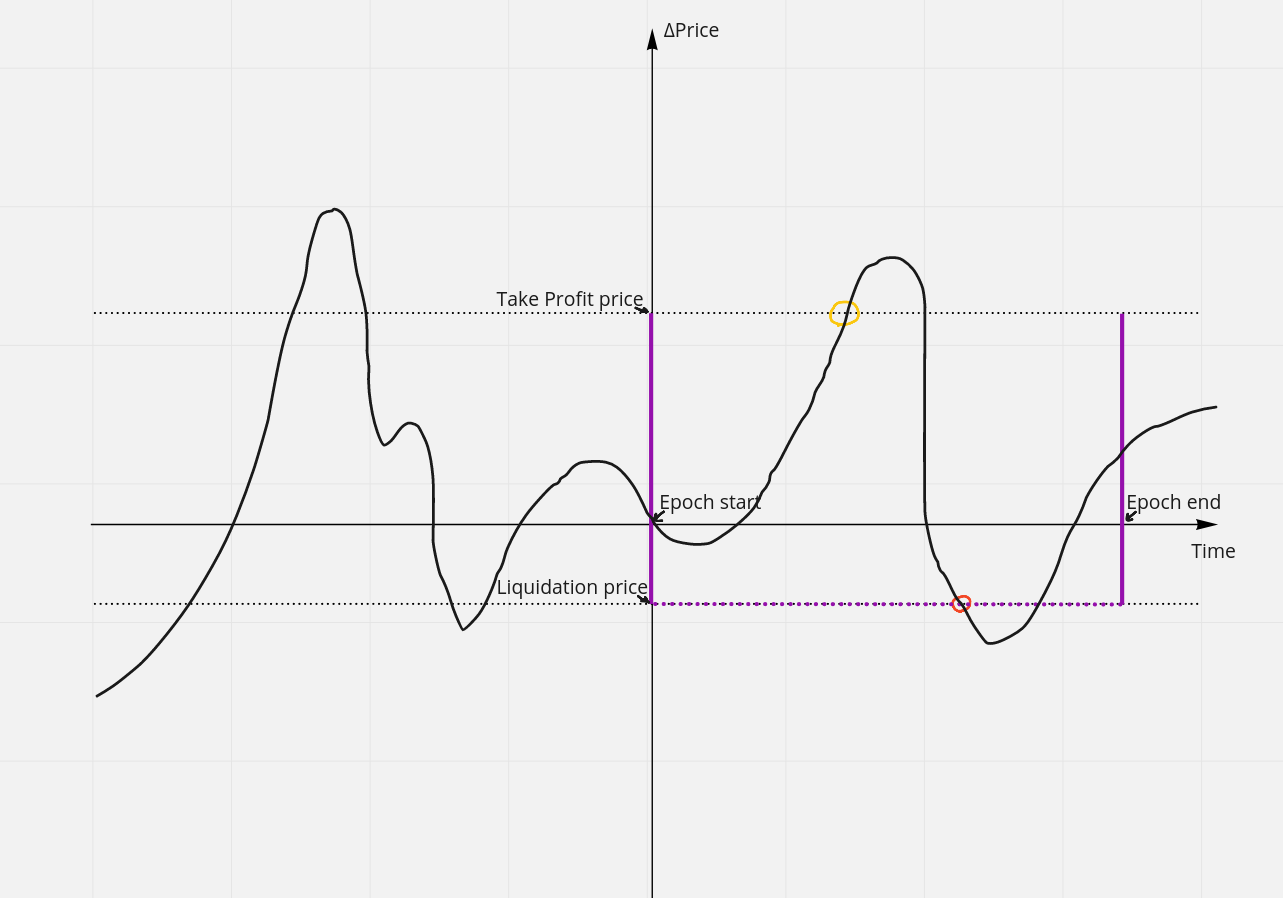
X axis is Time with 0 at the start of current liquifunding period.
Y axis is $Δ p$ from the price at liquifunding period starting timestamp.
Take Profit price is the $Δ p_{G}$ delta price level for the liquifunding period.
Liquidation price is $Δ p_{L}$ delta price level for the liquifunding period.
Orange circle is the first time Take Profit condition was satisfied. Red circle is the first time Liquidation condition was satisfied. In this case, the position should settle at Take Profit price, because it happened earlier.

The purple rectangular area is the area in question. At the end of the liquifunding period (see Section 8 for a precise definition of the time of execution), when the funding payments and borrow fee payments for that duration are made, a question needs to be answered:

Has the price intersected either the Take Profit or Liquidation price levels and, if so, which was first and at what timestamp?

One way to answer this question is to store price feed data in a data structure that can answer:

What is the first element of the data series that is greater (or lower) than a specific value?

That data structure must also support fast appending of new data points.

Fortunately, common blockchain storage mechanisms allow for gas-efficient querying of values. In particular, CosmWasm's de-facto standard storage library, cw-storage-plus, provides a Map data structure with a range method that allows us to find the first value before or after a given cut-off point, with gas costs being constant, or $O (1)$ complexity. Similarly, appending new data to this data structure is also $O (1)$ .

7.3. Liquidation and fee settling at end of liquifunding period

For a specific position $p os$ , the relevant period of time $T$ for which liquidatability and fee payments are made is defined as the intersection of the lifetime of the position and the liquifunding period.

Liquidatability is checked over $T$ . If the position became liquidatable for the first time at $t \in T$ , the position is settled with the price at $t$ . However, the fee rates are paid over the whole time period $T$ , and the delta neutrality fee is paid using the DNF rate at $T_{e n d}$ .

This is because the position is actually settled at a time $T_{e n d}$ . All the other positions and LPs may have been profiting from $p os$ paying funding and borrow fee rates over the whole duration $T$ , and $p os$ have been contributing to the protocol’s net notional size $N$ and utilization ratio $U_{t}$ .

In case the position has not been liquidatable over $T$ , funding payment and borrow fee payments are made for the position $p os$ , and all the relevant variables for that position $C_{p os}$ , $G_{p os}$ , $C_{min}$ , $p_{L}$ , $p_{G}$ are updated as explained in Sections 4 and 7.1.

7.4. External bots and blockchain congestion problem

An external bot (also referred to as a crank bot) is required to execute fee payments at regular intervals.

All positions are guaranteed to be well-funded to payout fees only if the external bot checks in regularly for each position. However, the bot mechanism is fallible due to server crashes, blockchain congestion, etc., and might miss execution for a period of time.

It would be unsatisfying to build a model that gives such strong guarantees, only to break them due to fees over blockchain congestion. An easy patch solution would be to increase margin collateral to cover a longer period of time.

However, in that case, the guarantee would lose its mathematical certainty and would have a caveat: potentially unbounded bad debt due to an unbounded period of time to clean up liquidated positions that are incurring fees.

The solution, described in Section 8, is to have an internal queue that tracks work that needs to be done for every price point. This allows the protocol to “retroactively” settle fees as work items are popped from the queue. This allows Well-funded Perps to keep the well-funded guarantee even in congestion scenarios of unbound but finite length.

8. State Staleness and Cranking

The protocol has several types of upkeep workloads that need to be be executed outside of user messages. These include closing positions that have either hit their liquidation or take profit price, settling outstanding funding and borrow fees, and settling price exposure.

8.1. Settling outstanding fees

All open positions have a liquidation margin which is defined to be enough for that position to pay the maximum possible fees (at their caps) over a specified period of time. This period of time is the sum of two protocol parameters: liquifunding period and the staleness time. External bots are responsible for querying at frequent, regular intervals to check if there is any work to be done, and if so, triggering the fee settlement for each position.

If cranking is not performed in time, the protocol enters a stale state. During a stale state, open, close and update messages are disallowed. This gives the protocol time to adjust by funding or liquidating positions which are not funded for that point in time before they incur higher funding payment PnL than the collateral locked in the positions.

Before a position is closed or updated, it always pays outstanding fees. This ensures that the position will pay from the timestamp it was opened until the timestamp it was closed.

8.2. Liquidating positions

For each new price update in the protocol, there may be some positions that have hit their liquidation or take profit price. All open positions are stored so that they can be efficiently iterated over for any given price update. In addition to funding all open positions, crank messages also iterate over all the price updates to close the liquidatable positions.

When liquidating a position, the price that is used to settle the trader and LP counter-side is the one that made that position liquidatable. It's important to note that this price may be slightly in the past due to cranking being an external process. The fees are paid up until the closing timestamp (or staleness timestamp if the protocol is stale) to ensure that there are exactly the same amount of funds received and payed through funding payments.

If the last processed price update is more than staleness time in the past, the protocol also becomes stale.

8.3. Cranking

A crank message is a permissionless message that executes the aforementioned workload. The only responsibility of external bots is to check if there is any crank work available to do in the protocol and to trigger it.

Crank messages cost gas, and so they require incentivization to be attractive to execute. Rewards for successfully executing a crank message must be at least greater than the gas spent on the execution. Funds used as rewards for successful cranking would be sourced from the yield fund. The upkeep cost of a position also add a condition on minimal size of a position that would be profitable for LPs to keep.

8.4. Staleness time

Timely execution of cranking messages is required for the healthy state of the protocol. If the crank is not processing work items fast enough, the protocol enters a stale state. This protects existing traders and liquidity providers by ensuring that every open position is well-funded for the full duration of their lifetime, even in the temporarily absence of cranking messages. This state should not be reached in normal conditions, and the cranking is permissionless and incentivized to increase resilience against centralized bots crashing.

To exit the stale state, crank messages need to be executed such that their workload timeline is advanced past the staleness timestamp. All funding of the positions and liquidations are done as if the block time is the staleness timestamp simulating cranking messages coming in just before the protocol became stale. This is possible because there are no trader messages executed, making these changes not retrospective relative to previous cranking and trader messages. Additionally, it ensures that positions are funded inside the funding time range.

9. Crypto denominated markets and off-chain notional

9.1. Delta-neutral staking rewards arbitrage strategy

Crypto assets with high staking rewards provide yield denominated in that crypto asset. It is possible to hedge the staked token price exposure, but the cost of the hedge is usually higher than the staking yield, making that trade unprofitable. However, if the cost was lower, it would be an arbitrage opportunity.

Since on Levana Perps it is possible to open a short position by borrowing only a part of the notional size of the trade, that hedged position could still be profitable, even if the borrow fee rate is higher than the staking yield. Borrow fee is paid on as little as 1/30th of the notional size.

The second ongoing cost to the hedged position is the funding fee rate. The more short positions that are opened, the higher the funding rate fee becomes, and this is the limiting factor on that trade.

The arbitrage would be between interest rates on debts denominated in US dollar and staking yield minus the costs to hedge, with funding rates acting as a price signal.

For example, if staking rewards on a token are 20% and arbitrageurs may source a 4% interest rate loan on US dollars/stablecoins, the borrow fee is 30%. That would make a hedged position profitable up to 20% - 4% - 30% * 1/30 = 15% funding fee rate.

9.2. Long positions staking rewards propagation as negative funding rates

Because of the attractive opportunity to hedge spot staked positions to create delta-neutral yield, there will be a persistent funding rate bias towards paying longs. This means that a reduced yield from staking rewards would be paid to long position holders on the notional size, which is the leveraged position size.

That would make the funding fee rate from the previous example leveraged up to: 10 * -15% = -150% for a 10x long position.

This gives the opportunity for long holders to not have to bypass staking rewards completely to trade on leverage.

In essence, long position holders would earn a premium to hold price exposure of the crypto asset for hedging arbitragers as funding rate fees.

9.3. Stablecoin denominated pair with off-chain notional index

For all assets native to the blockchain, there is a possibility of creating a crypto denominated pair with the notional asset being the US dollar, itself, instead of a particular stablecoin token. This removes the risk of the stablecoin depegging and bridge hack affecting the bridged version of the stablecoin.

For the bridged crypto assets like wETH or wBTC used as collateral in reverse pairs, the risk of the hack of the bridge remains, but the stablecoin depeg risk is eliminated.

Without a dependency on the notional asset being an on-chain crypto asset, there is the possibility of listing any notional index that has a corresponding reliable oracle price feed.

There is a dependency on cash-and-carries in making the liquidity provider pool roughly delta-neutral. Therefore, only notional indices that have deep liquidity in the spot market has low risks to LPs. The spot market must have a relatively cheap way to open and maintain long and short positions.

For example, it is possible to list a Gold notional index / USDC collateral asset trading pair.

This type of trading pairs allows Levana Well-funded Perps to list any notional index on any blockchain that has an on-chain stablecoin and oracle. If there is no stablecoin on the blockchain, it is still possible to list any notional index/native blockchain token. Any position in that pair can then be hedged with US / native blockchain token to remove exposure to the native blockchain token and only have exposure to the desired notional asset.

9.4. LP’s yield on crypto tokens in crypto denominated pairs

Crypto denominated Bitcoin pairs allow LPs to provide wBTC as a principal and receive in return yield that is also denominated in wBTC. That product does not include any stablecoin risks or the risk of any altcoin going bust.

The risks that LPs take are limited to protocol bug risks and Bitcoin / US dollar spot market meltdown risks. The yield is generated from leveraged traders paying a borrow fee with a risk premium.

This is the financial model of most companies providing yield on loaned crypto assets. However, LP for Levana Perps is a DeFi protocol, making it trustless and without the risks of centralized management of funds, which have materialized recently in insolvencies of companies with such a model.

Some of these companies became insolvent due to taking on risks of unrelated tokens or reusing collateral multiple times. Well-funded Perps provides a transparent and relatively simple model with a solution for the distressed market of Bitcoin and crypto lending.

Existing lending DeFi protocols are overcollateralized, which greatly reduces the meltdown risk, but it also reduces the yield of these protocols just as much.

9.5. Settlement of crypto denominated pair trading position equivalence

A reverse-direction position settlement on a crypto denominated pair is the same as settlement of a position in a stablecoin denominated pair.

Let us consider a trader who opens a position $pos$ in a stablecoin denominated pair with:

$C_{pos}$ collateral.
$N_{pos}$ notional size.
With leverage $l_{pos} = \frac{N_{pos}}{C_{pos}}\cdot p_o$.
At price $p_o$.
And closes it at price $p_c$ without liquidation or take profit.

Another trader opens a reverse position pos' $o n cry pt o d e n o mina t e d p ai r w i t h : *$ C_{pos'} = \frac{C_{pos}}{p_o} crypto collateral which is notional of stablecoin denominated pair.

$N_{pos'} = -p_o \cdot N_{pos} + C_{pos}$ reverse notional size.
With leverage $l_{pos'} = \frac{N_{pos'}}{C_{pos'}} \cdot \frac{1}{p_o} = \frac{-p_o \cdot N_{pos} + C_{pos}}{C_{pos}} \cdot p_o \cdot \frac{1}{p_o} = -\frac{N_{pos} \cdot p_o}{C_{pos}} + 1 = -l_{pos} + 1$.
At reverse price $\frac{1}{p_o}$.
And closes it at reverse price $\frac{1}{p_c}$.

Payouts to the traders of $pos$ and $pos_r$ circa fees are:

\[P_{pos} = C_{pos} + (p_c - p_o) \cdot N_{pos} = C_{pos} + p_c \cdot N_{pos} - p_o \cdot N_{pos}\] \[P_{pos'} = C_{pos'} + (\frac{1}{p_c} -\frac{1}{p_o}) \cdot N_{pos'} = \frac{C_{pos}}{p_c} - \frac{p_o \cdot N_{pos}}{p_c} + N_{pos}\]

Because payout $P_{pos'}$ is denominated in notional asset of the stablecoin denominated pair, by applying exchange ratio $p_c$ at close:

\[P_{pos'} \cdot p_c = C_{pos} + p_c \cdot N_{pos} - p_o \cdot N_{pos} = P_{pos}\]

This means that by opening a position in a crypto denominated pair with the same collateral value but in the notional denomination and with signed leverage $l_{pos'} = -l_{pos} + 1$, the trader’s payout profile is exactly the same, but with some difference in fees.

10. Risks, rewards, guarantees and fee size

With the protocol mechanics defined, we will explore the risks, rewards, guarantees, and fees that different market participants can take.

Traders get a strong, well-funded guarantee on profit and fees from liquidity providers. Liquidity providers give out these guarantees to traders and receive fees as yield in return for the risk taken to the provided principal.

The risks taken by liquidity providers scale with LPs’ exposure to the notional asset, which is the opposite of the net notional position of the traders. Therefore, the protocol has to maintain the net total notional traders’ position size roughly at 0.

Net notional is maintained with funding payments between traders (and capped delta neutrality fee, to a lesser extent).
Funding payments attract a special arbitraging type of trader using a cash-and-carry strategy. This strategy allows traders to enter a delta-neutral position, but still earn funding payments on the protocol, by opening a balancing reverse position on the spot market.
If that balance is not maintained, LPs’ rough delta-neutrality breaks and exposure to the notional asset is increased. That exposure may lead the LPs’ pool to experience risks in the form of a drawdown (or gain, if traders as aggregate lose).
Because the protocol does not need to defend its treasury with aggressive fee rates, the dynamic fee rate caps can be set significantly lower than on other perps protocols.

Another balance of the utilization ratio around target is maintained to keep the trader’s ability to open new positions with high capital efficiency.

Utilization ratio is balanced by gradually increasing or decreasing the borrow fee rate.
Borrow fee rate acts as the price at a point where demand for liquidity from traders meets the supply of that liquidity from providers.
If the utilization ratio hits close to 100%, traders may be unable to open new positions.

All of the market participants take on risks of bugs and hacks of the protocol infrastructure:

A bug in the implementation of the protocol.
A hack of bridge of the collateral asset if it is a bridged asset.
Oracle hack or downtime.
Blockchain downtime removing the ability to execute messages for closing the position.

10.1. Well-fundedness guarantee to the trader

A well-fundedness guarantee to the trader is the unique proposition of Well-funded Perps in leveraged trading. This guarantee can be written out as an inequality on the position’s PnL$ (profit or loss, positive when the position is in profit and negative otherwise).

10.1.1. Guarantee inequality derivation

First, let’s look at $PnL_{pos}$ has a lower bound on the time frame $T_e$ of one liquifunding period:

\[PnL_{pos} \ge \operatorname{clamp}(\Delta p \cdot N_{pos} - s_{pos} - F_{max},\ -C_{pos},\ G_{pos})\]

The lower bound is calculated assuming the maximum possible delta neutrality fee at close, the maximum possible funding payment and the maximum possible borrow fee payment over the liquifunding period $T_e$. Expanding the bounds from Sections 4.4.2, 4.5.2 and 7.1.2:

\[PnL_{pos} \ge \operatorname{clamp}(\Delta p \cdot |N_{pos}| - s_{cap} \cdot N_{pos} \cdot (p + \Delta p) - R_{f_{cap}} \cdot p_{max} \cdot T_e \cdot |N_{pos}| - R_{c_{cap}} \cdot T_e \cdot (G_{pos} + C_{pos}),\ -C_{pos},\ G_{pos})\]

And that can be expanded a bit further to use only the initial parameters of $pos$ and price $p$ into:

\[PnL_{pos} \ge \operatorname{clamp}((1 - s_{cap} \cdot \operatorname{sign}(N_{pos})) \cdot \Delta p \cdot N_{pos} - s_{cap} \cdot |N_{pos}| \cdot p - R_{f_{cap}} \cdot \max(p + \frac{G_{pos}}{N_{pos}}, p - \frac{C_{pos}}{N_{pos}}) \cdot T_e \cdot |N_{pos}| - R_{c_{cap}} \cdot T_e \cdot (G_{pos} + C_{pos}), -C_{pos},\ G_{pos})\]

The first part $(1 - s_{cap} \cdot \operatorname{sign}(N_{pos})) \cdot \Delta p \cdot N_{pos} - s_{cap} \cdot |N_{pos}| \cdot p$ is not dependent on the dynamic fees and is calculated precisely, while the second part $R_{f_{cap}} \cdot \max(p + \frac{G_{pos}}{N_{pos}}, p - \frac{C_{pos}}{N_{pos}}) \cdot T_e \cdot |N_{pos}| + R_{c_{cap}} \cdot T_e \cdot (G_{pos} + C_{pos})$ is an upper bound on dynamic fees to be paid.

That second part does depend on intermediate values of collateral that changes due to the fees in previous liquifunding periods. This complicates precisely writing down guarantee inequality for time frames longer than one liquifunding period.

However, it can be greatly simplified if we allow ourselves the assumption that the trader withdraws any possible positive funding payments he receives for position $pos$ at the end of each liquifunding period instead of “reinvesting” it into $C_{pos}$.

With that assumption, the guarantee for an arbitrary amount $n$ for a given liquifunding period is:

\[PnL_{pos} \ge \operatorname{clamp}((1 - s_{cap} \cdot \operatorname{sign}(N_{pos})) \cdot \Delta p \cdot N_{pos} - s_{cap} \cdot |N_{pos}| \cdot p - n \cdot (R_{f_{cap}} \cdot \max(p + \frac{G_{pos}}{N_{pos}}, p - \frac{C_{pos}}{N_{pos}}) \cdot T_e \cdot |N_{pos}| + R_{c_{cap}} \cdot T_e \cdot (G_{pos} + C_{pos})),\ -C_{pos},\ G_{pos})\]

10.1.2. Numerical examples of trader’s guarantee

The inequality has a lot of variables, but is not too complicated. Let us make some reasonable assumptions about the parameters of the trading pair:

Stablecoin collateral asset.
Delta neutrality cap $s_{cap}$ is at $0.5%$.
Liquifunding period length $T_e$ is 1 hour.
Funding rate cap $R_{f_{cap}}$ is at $30%$ annualized.
Borrow fee cap $R_{c_{cap}}$ is at $30%$ annualized.

And look at a couple of position examples:

Conservative longish-term bull $pos_1$ is a $2\times$ long position with $10\times$counter-side collateral leverage opened for 1 month with $$100$ in initial position value.

If price $p$ increased by $20%$, $pos_1$ is guaranteed to close with profit of at least $$11.57$. It is quite a bit less than perfect $$20$ of profit.

However, it is important to remember that this simulates the worst case scenario of an unrealistic unbalancing state of the protocol staying that way for the whole month. It includes only long positions being open, without any cash-and-carries, and without any new liquidity supply attracted by sky-high yields.

The trader was able to profit even in a worst-case scenario, despite not checking his position for a month and the trading pair being completely broken for all that time, because of a well-funded guarantee.
Short-term $10\times$ leverage short position $pos_2$ with $1\times$ counter-side leverage (to allow for huge max gains) targeting the top of the notional asset bursting and quickly going down to $0$ in a complete meltdown. The position is opened for 1 week and has an initial value of $$100$.

If the trader was able to open that position (meaning that liquidity providers did not see the meltdown coming) and timed the burst with 1 week precision, and if the price went down by $99%$ in that period of time, the trader would get $$982.04$ in profit, just $\approx $8$ shy of theoretically perfect $$990.00$.

10.1.3. Trader’s guarantee visualized on a payout chart

The guarantee can be visualized on a payout chart of the position at Open (red dashed line):

Untitled

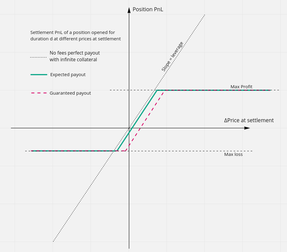
The $X$ axis is the $\Delta p$ and $Y$ axis is the position’s $PnL$ after a specified period of time.

The sloped dotted line is the $PnL$ of the position in a perfect world with $0$ fees of any kind and no liquidation or take profit prices.

Two horizontal lines are the max loss and max profit possible, achieved at liquidation or take profit prices of the position.

The green line is the expected $PnL$ of the position in the business-as-usual scenario. See Section 10.3 for numerical examples.

And lastly, the red line is the trader’s guaranteed payout.

At $\Delta p = 0$, perfect $PnL$ is also $0$. The expected payout is a bit shy of $0$ because of the fees, and the guaranteed $PnL$ is quite a bit lower at the lower bound for the worst-case market conditions scenario.

The slope of the red dashed line is just a little bit gentler than that of the perfect dotted line, with a ratio of $1 : (1-s_{cap})$ between the slopes. $1-s_{cap} = 0.995$ for the default delta neutrality cap, so the lines have a very similar slope in practice.

10.1.4. Risk-reward profile for traders

The purpose of opening a position is to gain exposure to the notional asset. For guaranteed exposure, traders pay fees. The exposure is the reward to the trader, while the only market condition risk that the trader takes on is the fees increasing from the expected fees up to respective caps, the magnitude of which was estimated.

This gives traders a clear framework to compare rewards and risks in order to make informed decisions. The relatively small magnitude of the effect of market risks on traders’ $PnL$ should make Well-funded Perps very dependable, even in bad market conditions.

10.2. Risks and risk-premium for LPs

LP and xLP tokens minted to liquidity providers represent a share of the LP pool and give the owner address the right to withdraw a pro-rata ratio of funds from the Yield fund that were collected during the time that the tokens were held.

The Yield fund portion that an LP is eligible to withdraw cannot be decreased, so it is not at risk. The principal in the LP pool, on the other hand, has a risk of impairment (as well as a chance to increase). The LP pool takes a net counter-position to all traders, including arbitrage bots.

The funding payment mechanism attracts arbitrage traders who bring the LP pool into rough delta-neutrality, significantly decreasing LPs’ exposure to the notional asset. This dynamic may break if the spot market of the trading pair becomes illiquid, putting arbitrage trades at risk. This is why a meltdown or a melt-up is the main risk to LPs. LPs would experience a large drawdown to their principal if:

The spot market becomes illiquid, putting arbitrage profitability at risk.
The price of the notional asset in the collateral asset moves by a significant amount.
The price moved in the direction benefiting most of the open interest in the trading pair.

10.2.1. Risks to LPs in a liquid market

Even in a liquid market with arbitrage bots active, a persistent slight delta non-neutrality is expected. Arbitrage bots will balance open interest up to a point of minimal profitability, but no further, leaving some non-zero funding and some delta non-neutrality.

The magnitude of that persistent non-neutrality can be estimated as $\frac{R_{f}}{K_f} \cdot \frac{\sum |N| \cdot p}{V_{\operatorname{LP}} + V_{\operatorname{xLP}}}$ — This is the funding rate divided by funding rates sensitivity and multiplied by total counter-side leverage. That non-neutrality, multiplied by the trading pair price volatility, would be the price risk that LPs take. The risk premium for that is expected to be included in the borrow fee rate.

10.2.2. Risks to LPs in an illiquid meltdown

In an illiquid market, when spreads increase, sensitivity skyrockets and liquidity is withdrawn. In the worst case scenario, in a total market meltdown, usual assumptions about arbitrage keeping the notional interest balance may break.

More specifically, if the delta neutrality fee on the spot market risks become greater than the profits from arbitrage, rational actors stop doing arbitrage. This leads to net notional interest moving away from a delta-neutral state, which on its own is not an impairment, but brings about an increase of market price exposure risks to LPs.

10.2.3. Inability to withdraw locked liquidity

In an illiquid market or when borrow fee is increasing, there is a risk of not being able to withdraw the provided liquidity in a timely manner, because all of it is locked in the trades. In this case, the borrow fee rate would be gradually increasing to attract more unlocked liquidity.

10.2.4. Risk premium for providing liquidity

All of these risks are assessed by liquidity providers. From the emergent behavior of LPs and traders, a fair borrow fee would be found, which includes risk premiums for unconditionally entering counter-positions and taking risks of the market going illiquid.

10.3. Expected fees estimation

In Sections 10.1 and 10.2, the guarantees and risks of the worst case scenario for traders and LPs were shown. Let us now explore the expected fee rates of a balanced protocol.

Trading pairs with an asset that allows for high staking yield in that asset have a persistent bias of funding rates being paid to longs because of the arbitrage opportunities described in Section 9. Funding rates estimation is derived from that arbitrage profitability. Other trading pairs will have funding rates around zero. There, funding rates are derived with the usual cash-and-carry strategy profitability.

Borrow fee is derived from estimating the risk premiums that needs to be covered for LP to become attractive.

10.3.1. Expected fees derivation for assets without staking

Funding rates will be set such that performing a cash-and-carry strategy would yield a low profit.

Borrow fee rates will be set such that they covers all risk, including risk-premiums, and also the risk-free yield on the collateral.

Cash-and-carry trade having profit margin $M$:

\[ Payout_{c\&c} = \overline{R_f \cdot p} \cdot N \approx \overline{R_f} \cdot \frac{L_{max}}{1+L_{max}} \cdot C \]

\[ Payout_{c\&c} = (1 + M) \cdot Cost_{c\&c} \]

\[ Cost_{c\&c} = Fee_{trading} + \overline{R_c} \cdot \frac{C}{1+L_{max}} + R_{loan} \cdot \frac{L_{max}}{1+L_{max}}\cdot C - s_{c\&c} \]

\[ Fee_{trading} = Fee_N \cdot n \cdot \frac{L_{max}}{1+L_{max}} \cdot C + \frac{1}{1+L_{max}} \cdot Fee_G \approx n \cdot Fee_N \cdot C \]

\[ s_{c\&c} > 0 \]

\[ Cost_{c\&c} \approx C \cdot (Fee_N \cdot n + \frac{\overline{R_c}}{1+L_{max}} + \frac{L_{max}}{1+L_{max}} \cdot R_{loan}) \]

\[ \overline{R_f} \approx (1+M) \cdot (Fee_N \cdot n \cdot \frac{1+L_{max}}{L_{max}} + \frac{\overline{R_c}}{L_{max}} + R_{loan}) \]

Where:

$n$ — expected number of popularity of short/long open interest reversals per year.

The borrow fee as yield that providers will demand to cover:

The risk free rate that LPs pass up by locking collateral with Perps instead of other risk-less places, such as US treasuries for USD or overcollateralized loans.
The risks that LPs would collectively ascribe to a market meltdown, multiplied by expected drawdown in the notional asset as illiquidity risk.
The risks of bugs or bridge hacks, multiplied by 100% drawdown in that scenario.
Compensation for the persistent delta neutrality ratio bias. The compensation is the delta non-neutrality multiplied by the notional asset volatility.

\[ \overline{R_c} \approx (R_{risk\_free} + R_{illiquidity} + R_{bug} + \frac{\overline{|R_f|}}{K_f} \cdot \sigma_N - R_{trading\_fees}) \cdot \frac{1}{1 - Y_{DAO}} \]

Where

$Y_{DAO}$ is the flat percentage of the Yield fund that DAO gets as profits.
$\sigma_N$ is the volatility of the notional asset.

\[ \overline{R_f} \approx (1+M) \cdot (Fee_N \cdot n \cdot \frac{1+L_{max}}{L_{max}} + R_{loan})+ \frac{(1+M)}{L_{max}}\cdot\overline{R_c} \]

\[ \overline{R_c} \approx (R_{risk\_free} + R_{illiquidity} + R_{bug} - R_{trading\_fees}) \cdot \frac{1}{1 - Y_{DAO}} + \frac{\sigma_N}{K_f \cdot (1-Y_{DAO})} \cdot \overline{|R_f|} \]

This is a system of two linear equations with two variables. It can be solved after making assumptions on all the parameters and all the market conditions.

10.3.2. Numerical fee estimations for assets without staking

Assuming these parameters for a USD/wBTC trading pair:

$M=40%$ profit margin for cash and carries.
$n=12$ cash and carry trades per year.
$Fee_N = 0.05%$ trading fees on notional size.
$L_{max} = 30$ max leverage.
$R_{loan} = 4.5%$ cash and carries being able to loan unlimited amount of collateral asset at that interest rate.
$R_{risk\_free} = 3.5%$ risk-free return on collateral asset.
$R_{illiquidity} = 3%$ probability of the notional asset spot market going illiquid per year multiplied by the size of the illiquid price move.
$R_{bug} = 3%$ probability of a catastrophic bug / exploit in the infrastructure and the protocol.
$R_{trading\_fees} = 5%$ expected LP yield from fees. Hard to estimate without knowledge of the total volume to open interest ratio.
$\sigma_N = 120%$ annualized volatility of the notional asset.
$K_f = 5$ sensitivity of the funding rates.
$Y_{DAO} = 10%$ part of Yield fund as profit for the DAO.

Gives:

$\overline{R_f} = 7.5%$ expected annualized funding rate.
$\overline{R_c} = 7.0%$ expected annualized borrow fee rate.

10.3.3. Expected fees derivation for assets with high staking yield

For borrowing USD for $R_{loan}$ and staking the collateral asset for a higher $R_{stake}$:

\[ R_{stake} \cdot \frac{L_{max}}{1+L_{max}} \cdot C - R_T \cdot C = \overline{R_f} \cdot \frac{L_{max}}{1+L_{max}} \cdot C + Fee_{trading} \cdot n \cdot \frac{L_{max}}{1+L_{max}} \cdot C + \overline{R_c} \cdot \frac{1}{1+L_{max}} \cdot C + R_{loan} \cdot C \]

\[ R_{stake} - R_T \cdot \frac{1 + L_{max}}{L_{max}} = \overline{R_f} + Fee_{trading} \cdot n + \frac{\overline{R_c}}{L_{max}} + \frac{(1+L_{max})\cdot R_{loan}}{L_{max}} \]

\[ \overline{R_f} = R_{stake} - R_T \cdot \frac{1 + L_{max}}{L_{max}} - Fee_{trading} \cdot n - \frac{(1+L_{max})\cdot R_{loan}}{L_{max}} - \frac{\overline{R_c}}{L_{max}} \]

Borrow fee is calculated the same way:

\[ \overline{R_c} \approx (R_{risk\_free} + R_{illiquidity} + R_{bug} + \frac{\overline{|R_f|}}{K_f} \cdot \sigma_N - R_{trading\_fees}) \cdot \frac{1}{1 - Y_{DAO}} \]

10.3.4. Numerical fee estimations for assets with high staking yield

Assuming these parameters for a USD/OSMO trading pair, estimated from OSMO staking with validators for 26% yield:

$Y_{target}=5%$ profit margin for arbitragers between spot staking and short Perps hedging.
$n=12$ cash and carry trades per year.
$Fee_N = 0.05%$ trading fees on notional size.
$L_{max} = 30$ max leverage.
$R_{loan} = 4%$ cash and carries being able to loan unlimited amount of collateral asset at that interest rate.
$R_{risk\_free} = 26%$ risk-free return on collateral asset.
$R_{illiquidity} = 5%$ probability of the notional asset spot market going illiquid per year multiplied by the size of the illiquid price move.
$R_{bug} = 3%$ probability of a catastrophic bug / exploit in the infrastructure and the protocol.
$R_{trading\_fees} = 10%$ expected LP yield from fees. Hard to estimate without knowledge of the total volume to open interest ratio.
$\sigma_N = 200%$ annualized volatility of the notional asset.
$K_f = 5$ sensitivity of the funding rates.
$Y_{DAO} = 10%$ part of Yield fund as profit for the DAO.

Gives:

$\overline{R_f} = -19.3%$ expected annualized funding rate — long position holders are estimated to get that rate paid on their leveraged up position size.
$\overline{R_c} = 35%$ expected annualized borrow fee rate on counter-side collateral.

Total fees paid or received by long position holders as an APR from the collateral used to open the position:

Total fees for longs	2x	5x	10x	30x
Levana - OSMO Uncapped	15.75%	63.01%	141.77%	456.80%
Levana - OSMO 5x max gains	5.63%	-7.79%	-70.63%	-422.65%
Levana - OSMO 10x max gains	9.85%	15.81%	-17.53%	-313.11%

Where a negative number indicates a total negative fees, paying the holder of the long position.

Levana Well-funded Perps is a leveraged spot-price well-funded collateral-settled perpetual swaps protocol. It introduces a novel way to delineate risk between market participants. The incentive structure offers a risk premium to liquidity providers who take on the spot market illiquidity risk.

Traders get strong guarantees for settlement in any future market conditions with a very low liquidation margin ratio.
Liquidity Providers receive roughly delta-neutral yield for taking on spot market meltdown risk. That yield is found in a free market of supply and demand for liquidity to be used as collateral.
The protocol does not require a risk fund, and DAO Treasury has no insolvency risk.

The absence of native price discovery in spot-price settled perps is addressed by introducing a Capped Delta Neutrality Fee mechanism.

Levana Perps Documentation